Scaling and Encoding Are Not Cleaning: Getting the Order of Data Prep Right
Why scaling and one-hot encoding belong after cleaning and the train/test split, with the right order of steps and examples in DuckDB SQL and pandas.
By Tnas · Published · 7 min read
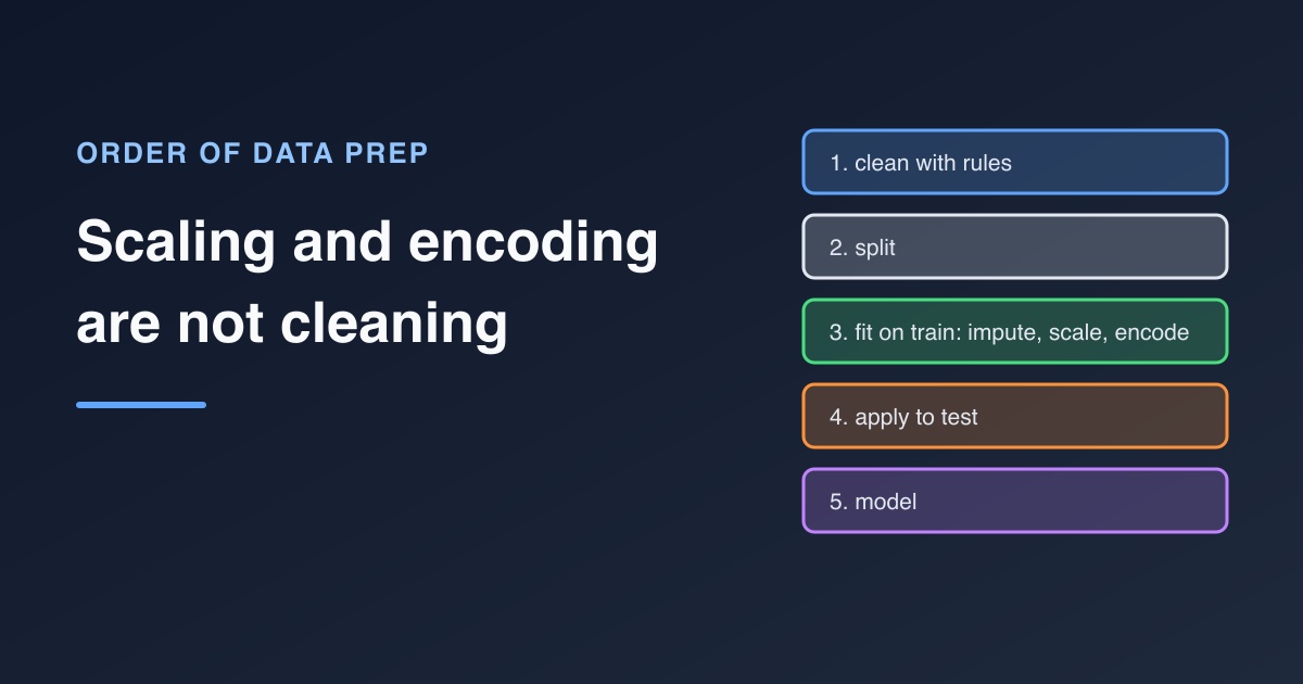
Cleaning means making data correct: right types, real missing values, no duplicates, approved categories. Scaling and encoding are the steps that make correct data convenient for one particular model: numbers on a similar range, categories turned into columns. So the order is fixed: clean all rows with written rules, split into training and test data, then fit imputers, scalers and encoders on the training rows only and apply them unchanged to the test rows. Scaled and encoded values never go back into the shared clean table. The examples below show, in DuckDB SQL and pandas, what goes wrong when the order slips.
Key Takeaways
- Cleaning fixes errors and is shared by every use of the data. Scaling and encoding are model-specific representations and belong in the model's pipeline, not in the clean table.
- The safe order is: clean, deduplicate, split, then fit imputation, outlier handling, encoding and scaling on training rows, then model.
- Scaling before the split leaks test data. In the example, including the two test-period orders (one of them 300.0) moved the mean from 30.0 to 70.71 and the standard deviation from 7.91 to 101.47.
- Encoding before categories are cleaned turns every typo into its own column. Encoding fitted on training data must handle categories that only appear later.
What counts as cleaning, and what doesn't?
The useful test is whether a step makes the data more true or more convenient.
| Step | Cleaning or preparation? | Learned from data? | Where it runs |
|---|---|---|---|
| Parse types, dates and ids | Cleaning | No | Before the split, all rows |
| Blanks and sentinel codes to missing | Cleaning | No | Before the split, all rows |
| Trim, fix encoding, map categories with a dictionary | Cleaning | No | Before the split, all rows |
| Remove exact duplicates | Cleaning | No | Before the split, all rows |
| Validate ranges, flag outliers with reasons | Cleaning | No (written rules) | Before the split, all rows |
| Fill missing values with a median | Preparation | Yes | After the split, fit on train |
| Cap outliers at a percentile | Preparation | Yes | After the split, fit on train |
| One-hot or ordinal encoding | Preparation | Yes (the category list) | After the split, fit on train |
| Standardise or min-max scale | Preparation | Yes (mean, standard deviation, min, max) | After the split, fit on train |
Cleaning steps are rules: they give the same answer for a row whatever other rows exist, so they are safe on the whole dataset. Preparation steps learn numbers or lists from the data, which makes them part of the model. The guide to avoiding leakage in data preparation covers this boundary in detail, and the data cleaning checklist lists the cleaning half.
This post is about the order of those steps and the fit-on-train mechanics. The companion posts on data cleaning versus data transformation and data cleaning for machine learning cover the definitions and the wider changes ML brings.
There is a practical reason to keep them apart too. A cleaned order_value of 35.0 means 35 currency units to everyone who reads it. A scaled value of 0.63 means "0.63 standard deviations above the training mean of one model", and it changes every time the model is retrained. Writing it into a shared table makes the table harder to use and ties it to one model's history.
Mistake 1: Scaling before the split
Standardising subtracts a mean and divides by a standard deviation. Both are learned from data, so computing them on all rows lets the test set shape the training features. Here are seven orders, trained on January and February and tested on March, with one large March order:
CREATE TABLE orders AS SELECT * FROM (VALUES
 (1, DATE '2026-01-05', 'web',   20.0),
 (2, DATE '2026-01-12', 'store', 35.0),
 (3, DATE '2026-01-20', 'web',   25.0),
 (4, DATE '2026-02-03', 'store', 40.0),
 (5, DATE '2026-02-17', 'web',   30.0),
 (6, DATE '2026-03-02', 'phone', 300.0),
 (7, DATE '2026-03-09', 'web',   45.0)
) AS t(order_id, order_date, channel, order_value);

SELECT 'all rows' AS fitted_on, round(avg(order_value), 2) AS mean_value,
       round(stddev_samp(order_value), 2) AS sd_value FROM orders
UNION ALL
SELECT 'train only', round(avg(order_value), 2), round(stddev_samp(order_value), 2)
FROM orders WHERE order_date < DATE '2026-03-01';
┌────────────┬────────────┬──────────┐
│ fitted_on  │ mean_value │ sd_value │
├────────────┼────────────┼──────────┤
│ all rows   │      70.71 │   101.47 │
│ train only │       30.0 │     7.91 │
└────────────┴────────────┴──────────┘
Fitted on all rows, every training order would be scaled against a mean of 70.71, pulled up almost entirely by one March order the model is supposed to have never seen. The correct version learns the parameters from training rows and applies them to every row:
WITH params AS (
  SELECT avg(order_value) AS mu, stddev_samp(order_value) AS sigma
  FROM orders WHERE order_date < DATE '2026-03-01'
)
SELECT order_id,
       CASE WHEN order_date < DATE '2026-03-01' THEN 'train' ELSE 'test' END AS part,
       order_value,
       round((order_value - mu) / sigma, 2) AS order_value_scaled
FROM orders CROSS JOIN params
ORDER BY order_id;
┌──────────┬───────┬─────────────┬────────────────────┐
│ order_id │ part  │ order_value │ order_value_scaled │
├──────────┼───────┼─────────────┼────────────────────┤
│        1 │ train │        20.0 │              -1.26 │
│        2 │ train │        35.0 │               0.63 │
│        3 │ train │        25.0 │              -0.63 │
│        4 │ train │        40.0 │               1.26 │
│        5 │ train │        30.0 │                0.0 │
│        6 │ test  │       300.0 │              34.15 │
│        7 │ test  │        45.0 │                1.9 │
└──────────┴───────┴─────────────┴────────────────────┘
Order 6 scales to 34.15, far outside anything in training. That isn't a bug in the scaling. It is an honest signal that production can send values the model hasn't seen, which the leaky version would have hidden. The scikit-learn documentation states the general rule as "never call fit on the test data" (scikit-learn, Common pitfalls), and the split train and test by time exercise practises the split itself.
Mistake 2: Scaling before handling outliers
Mean and standard deviation are pulled by extreme values, so the order of outlier handling and scaling matters even within the training rows. If one training value is extreme, standardising squeezes every normal value into a narrow band. Here is the training data with the 300.0 order moved into it, scaled two ways:
WITH train AS (
  SELECT * FROM (VALUES (20.0), (35.0), (25.0), (40.0), (30.0), (300.0)) AS t(order_value)
),
params AS (
  SELECT avg(order_value) AS mu, stddev_samp(order_value) AS sigma,
         median(order_value) AS med,
         quantile_cont(order_value, 0.75) - quantile_cont(order_value, 0.25) AS iqr
  FROM train
)
SELECT order_value,
       round((order_value - mu) / sigma, 2) AS standard_scaled,
       round((order_value - med) / iqr, 2) AS robust_scaled
FROM train CROSS JOIN params
ORDER BY order_value;
┌─────────────┬─────────────────┬───────────────┐
│ order_value │ standard_scaled │ robust_scaled │
├─────────────┼─────────────────┼───────────────┤
│        20.0 │            -0.5 │          -1.0 │
│        25.0 │           -0.45 │          -0.6 │
│        30.0 │           -0.41 │          -0.2 │
│        35.0 │           -0.36 │           0.2 │
│        40.0 │           -0.32 │           0.6 │
│       300.0 │            2.04 │          21.4 │
└─────────────┴─────────────────┴───────────────┘
With standard scaling, the five normal orders land between -0.5 and -0.32, so a 20-unit difference in value becomes a difference of less than 0.2. Scaling with the median and interquartile range keeps them spread from -1.0 to 0.6 and leaves the outlier clearly separate. scikit-learn's preprocessing guide warns that "if your data contains many outliers, scaling using the mean and variance of the data is likely to not work very well" and suggests RobustScaler, which uses the median and interquartile range instead (scikit-learn, Preprocessing data).
The order that works:
- During cleaning: flag outliers with a reason and fix values that break domain rules. The outliers: flag, don't delete guide covers this.
- After the split: if the model needs it, cap values at percentiles learned from training rows, or use a robust scaler.
- Then scale.
Mistake 3: Encoding before categories are clean
One-hot encoding creates one column per distinct value. If the category column still contains Web, 'web ' (with a trailing space) and wbe, encoding produces three columns for one channel, and the model has to learn the same thing three times from a third of the data each. Normalising and mapping categories with an approved dictionary is a cleaning step and must happen first; cleaning categorical data and the map channels with an approved dictionary exercise cover it.
Mistake 4: Encoding without a fixed category list
Even with clean categories, encoding is learned: the list of columns comes from the data it was fitted on. In the example, training contains only web and store, while the test period adds phone. Encoding each part separately with pandas produces different columns:
import pandas as pd

df = pd.DataFrame({
    "order_date": pd.to_datetime(["2026-01-05", "2026-01-12", "2026-01-20", "2026-02-03",
                                  "2026-02-17", "2026-03-02", "2026-03-09"]),
    "channel": ["web", "store", "web", "store", "web", "phone", "web"],
})
train = df[df["order_date"] < "2026-03-01"]
test = df[df["order_date"] >= "2026-03-01"]

train_x = pd.get_dummies(train["channel"], prefix="channel")
test_x = pd.get_dummies(test["channel"], prefix="channel")
print(list(train_x.columns), list(test_x.columns))

test_x = test_x.reindex(columns=train_x.columns, fill_value=False)
print(test_x)
['channel_store', 'channel_web'] ['channel_phone', 'channel_web']
   channel_store  channel_web
5          False        False
6          False         True
The test matrix has a channel_phone column the model has never seen and is missing channel_store, so the model would either fail or, worse, read columns in the wrong positions. Reindexing to the training columns fixes the shape: the phone order becomes all False, meaning "none of the known channels". scikit-learn's OneHotEncoder does the same with handle_unknown='ignore'; with handle_unknown='infrequent_if_exist' it maps unknowns to the infrequent category if one was learned, and otherwise to all zeros (scikit-learn, OneHotEncoder). pandas' own get_dummies has no memory of the training columns, which is why the reindex step is needed. Categories that only appear after training are the reason to fit the encoder once, on training data, and reuse it; the categories the model never saw exercise practises this.
Where imputation and indicators fit
Missing values sit on both sides of the line. Turning blanks, N/A and -1 into real missing values is cleaning, done on all rows. Filling those missing values with a median is preparation, fitted on training rows. Two ordering details matter:
- Create the missing-value indicator before filling, or the information about which values were missing is gone.
- Impute before scaling when the scaler can't accept missing values, and fit both on the same training rows so the filled values are scaled consistently.
The fill gaps without leakage and impute with an indicator column exercises practise both steps.
Keep the fitted steps together
The easiest way to keep the order right is to put every learned step in one object that is fitted once on training data and saved with the model. In scikit-learn that is a Pipeline, often with a ColumnTransformer that applies an imputer and scaler to numeric columns and an encoder to categorical ones. scikit-learn recommends pipelines because they make it harder to forget a transformation and keep each cross-validation fold from seeing the others' data (scikit-learn, Common pitfalls). In SQL, the equivalent is a small parameters table (means, standard deviations, category lists) computed from training rows and joined to every later batch.
The clean table stays upstream of all of this, versioned and model-agnostic. The reproducible cleaning pipelines guide covers how to keep that part repeatable.
The order, in one list
- Parse types and turn blanks, placeholders and sentinel codes into missing values.
- Trim, fix encodings and map categories with an approved dictionary.
- Remove exact duplicates and validate ranges, flagging outliers with reasons.
- Save this as the clean table.
- Split into training and test data (by time when predicting the future).
- On training rows, fit: missing-value indicators and fill values, outlier caps, encoders, scalers.
- Apply the fitted steps unchanged to test and production rows.
- Train and evaluate the model.
Frequently asked questions
Should you scale data before or after the train/test split?
After. The mean, standard deviation, minimum and maximum used for scaling are learned from data, so they must come from training rows only and then be applied unchanged to the test rows. Scaling first lets test data influence training features.
Is one-hot encoding part of data cleaning?
No. It changes how clean categories are represented for a model, and the list of columns is learned from training data. Cleaning the categories themselves, such as fixing case, typos and synonyms, is cleaning and comes first.
Should you impute missing values before or after scaling?
Usually impute first, after creating a missing-value indicator, because many scalers and models can't accept missing values. Fit both steps on the training rows only.
Do all models need scaled features?
No. Scaling matters for models that compare distances or use gradient-based training on raw magnitudes, such as k-nearest neighbours, support vector machines and regularised linear models. Decision trees split on thresholds of one feature at a time, so they are unaffected by monotonic rescaling.
Sources
- scikit-learn developers, Common pitfalls and recommended practices, retrieved 2026-11-05.
- scikit-learn developers, Preprocessing data, retrieved 2026-11-05.
- scikit-learn developers, sklearn.preprocessing.OneHotEncoder, retrieved 2026-11-05.
- pandas developers, pandas.get_dummies, retrieved 2026-11-05.
- DuckDB, Aggregate functions, version 1.5 (
avg,stddev_samp,quantile_cont), retrieved 2026-11-05.